Lab. 7. Stability analysis of the Ricker's model
Ricker's model simulate the dynamics of a population with intra-specific competition. It is a discrete-time analog of the logistic model. Ricker's model is:
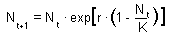
where K is carrying capacity (=equilibrium density) and r is the intrinsic rate of population increase. Use Microsoft Excel to simulate population dynamics with the Ricker's model. In all simulations, the carrying capacity K= 1000.
1.Run the model with r=0.2 for 80 generations starting from No = 1. Plot the graph, explain why it has the S-shape.
2.Estimate relaxation time (time until the population density approaches the equilibrium with specific accuracy, e.g., 0.1) as a quantitative measure of stability. Run the model with parameter r=0.05; 0.1; 0.2, 0.3;... 1.9, 1.95 and find relaxation time using No = 900 as initial density. Plot relaxation time versus r and explain the shape of the graph. Note: the number of generations should be greater than the relaxation time.
3. Run the model with parameter r changing from 1.8 to 3.0 with step 0.025 and plot the bifurcation diagram as follows. Run the model for 200 generations with each value of r, discard first 100 generations and plot population numbers in the final 100 generations versus the r-value. Describe the plot: at what value of r the population dynamics changes from a stable equilibrium to a 2-point limit cycle, to a 4-point limit cycle, to chaos? Plot population dynamics versus time for r=l; r=1.8; r=2.2; r=2.6; r=2.8. Indicate the type of population dynamics.
4. Add random fluctuations to the model:
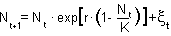
where  is a random variable with normal distribution, mean = 0 and standard deviation = s. The random variable with normal distribution (m =0, and SD=1) can be obtained by summing 12 random number (function RAND()) with the uniform distribution ranging from 0 to 1 and subtracting 6 from the sum. Run the model with parameter r changing from 0.1 to 1.9 with 0.1 steps, K=1000, s=10, No = 1000, for 500 generations. Estimate the coefficient of v-stability:
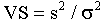 . Compare the graph with the graph of relaxation time.


