Petri Nets
A more universal factor-process model was developed by Petri (1962). He introduced a class of nets which later were named "Petri nets". These nets have two types of components: positions and transitions (positions = factors, transitions = processes).

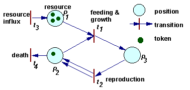
Example of a Petri net
The dynamics of a Petri net is a sequence of transition "firing". When a transition is fired then 2 things happen. First, tokens are taken away from positions which have arrows going from these positions to the transition considered. If more than 1 arrow goes from position to transition, then the number of tokens removed from that position is equal to the number of arrows. Second, new tokens are placed on positions indicated by arrows that originate from the transition. The number of tokens placed corresponds again to the number of arrows (in the case of multiple arrows).
For example, in the figure above, when transition t1 is fired, then 1 token is removed from position p1, 1 token is removed from position p2, and 1 token is added on position p3. When transition t2 is fired, then 1 token is removed from position p3, and 1 token is added on position p2. Transition t1 can be interpreted as feeding and growth, and transition t2 as reproduction.
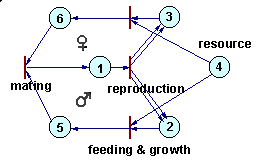
Petri nets can be used to simulate complex ecological interactions within a population and among populations. The figure below is an example of a population with sexual reproduction. More examples can be found in Sharov (1991).

Petri net representing a population with sexual reproduction
The rate of processes is not defined within a Petri net, it should be specified separately. The rate of chemical reactions is usually defined by mass action law. Mass action law is used in many population ecology models (exponential growth, Lotka-Volterra eqns.). However, there are much more cases in ecology than in chemistry when mass action law does not work. In these cases, the rate of equations is defined in some different way.
How to write differential equations from the Petri net:
1. Write left sides of differential equations for each position i:
dxi/dt=
2. For each process (transition)
t do the following:
a. Estimate process rate Vt
= ktxi
xj ... where kt
is a constant and xi, xj
are the number of tokens in
starting positions i, j,... for
this process.
b. Subtract Vt
from dxi/dt
for each starting position i
c. Add Vt to dxi/dt
for each ending position i.
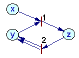
Example:

Rates of processes 1 and 2:

Rates of change in token numbers:

Other examples:
 V = k
V = k
 V = kx
Coefficient k depends on the rate of organisms' movement (=temperature). Mass action law assumes that particles move incessantly. However, organisms are not like gas molecules. Predators stop hunting after saturation. A similar saturation effect exists in macromolecules (enzymes). In these cases, mass action law should be replaced by Michaelis-Menton equation: V = kxy/(1+ax). The rest of the algorithm remains the same.
Effect of other factors (temperature, age, sex, etc.) can be expressed as variation of coefficient k. As a result, k will become a function of several variables.


