1.3. Population system

The term "life-system" was introduced by Clark et al. (1967). Later, Berryman (1981) suggested another term "population system" which is definitely better. A short review of the life-system methodology was published by Sharov (1991).

Major components of a population system

1. Population itself. Organisms in the population can be subdivided into groups according to their age, stage, sex, and other characteristics.
2. Resources: food, shelters, nesting places, space, etc.
3. Enemies: predators, parasites, pathogens, etc.
4. Environment: air (water, soil) temperature, composition; variability of these characteristics in time and space.

Temporal and spatial structure of a population system

Dynamics of Population Systems

Factor-Process concept: Environmental factors do not affect population density directly, instead they affect the rate of various ecological processes (mortality, reproduction, etc.) which finally result in a change of population density. Processes can change the value of factors; thus, feedback loops become possible.
Advantage: Can handle complex dynamic interactions among components of population systems including time-delays, negative and positive feedbacks.

In 50-s and 60-s there was a discussion about population regulation between two schools in population ecology. An agreement could not be reached because these schools used different concepts of population dynamics. Andrewartha and Birch (1954) used the factor-effect concepts whereas Nicholson (1957) used the factor-process concept.

The factor-process concept works not only in population ecology but in any kind of dynamic systems, e.g. in economic systems. Forrester (1961) formalized the factor-process concept and applied it to industrial dynamics. Later this formalism became very popular in ecology and is widely used especially in ecosystem modeling.

The model of Forrester is based on tank-pipe analogy. The system is considered as a set of tanks connected by pipes with vents which can regulate the "flow" of liquid from one tank to another. The flow of "liquid" between tanks is considered as "material flow". However there is also "information flow" that regulates the vents. Vents are equivalent to processes; and the amount of liquid in a tank is a variable or a factor because it can affect processes via information flow.

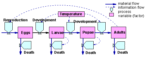
The figure above is the Forrester diagram for an insect population system with 4 stages: eggs, larvae, pupae, and adults. Transition between these states (development) is regulated by temperature. Influx of eggs depends on the number of adults. Mortality occurs in all stages of development. Larval and pupal mortality is density-dependent.

Diagrams of Forrester can be easily transformed into differential equation models. Each process becomes a term in a differential equation that determines the dynamics of the variable. For example, the number of larvae in the figure above is affected by 3 processes: egg development ED(T), larval development LD(T), and larval mortality LM(N). Egg and larval development rates are functions of temperature T; whereas larval mortality is a function of larval numbers N. The equation for larval dynamics is the following:

Here the term ED(T) is positive because egg development increases the number of larvae ("liquid" influx). Terms LD(T) and LM(N) are negative because larval development (molting into pupae) and mortality reduce the numbers of larvae.

Limitations of Forrester's model:

1. Distinction between information and material flows was not clear because information cannot be transferred without any matter. For example: egg or seed production is not only an information flow, there is a flow of matter too.
2. Only one type of processes is considered in which "fluid" moves from one tank to another. This is good representation of organisms changing their state. However, it is impossible to apply the model to the processes that involve two or more participants. For example, when a parasite enters a host then it is impossible to make a "pipe" that starts from two "tanks": host and parasite, and ends in the "tank" of "parasitized host".
3. Only one level of processes is considered. In some cases it is important to consider processes at two spatial levels, e.g., the dynamics of phytophagous insects can be considered within a host plant and within a population of host plants.

Factors and processes

Components of the system will be called factors because they affect system dynamics. The state of the component is the value of the factor. Factors are considered with as many details as necessary for understanding system's dynamics.

Examples of factors:

• In simple models (e.g., exponential or logistic), there is only one factor (=component): the population itself. Its value is population density.
• In age-structured populations, each age class is a factor and its value is equal to the density of individuals in that class.
• Natural enemies and various resources can be considered as additional factors. Then, the abundance of predators, parasites, or food will be values of these factors.
• Weather can be viewed as a set of factors: temperature, precipitation, etc. Each of these factors has a numerical value.
• Factors may have a hierarchical structure. If the population occupies multiple patches in space, then all factors (e.g., population density, density of natural enemies and resources, temperature) become patch-specific.

Examples of processes

• The birth of an organism is an event. The birth rate is the number of births per unit time. The specific birth rate (= reproduction rate) is the birth rate per 1 female (or per 1 parent).
• Death of an organism is an event. Mortality on a specific stage from a specific cause (e.g., parasitism, predation, starvation) is a process. Mortality rate is the number of deaths per unit time. Specific mortality rate is the number of deaths per unit time per organism.
• Other processes are: growth, development, consumption of resources, dispersal, entering diapause, etc.

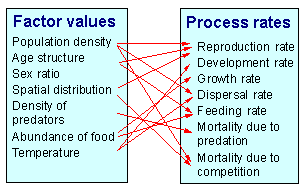
Factors affect the rate of processes as shown below:

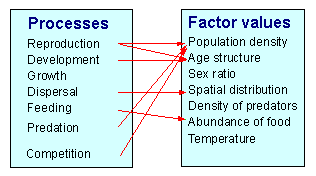
On the other hand, processes change the values of factors:

A process may be affected by multiple factors. For example, mortality caused by predation may depend on the prey density, predator density, number of refuges, temperature (if it changes the activity of organisms), etc.

The value of a factor may change due to multiple processes. For example, the number of organisms on a specific stage changes due to development (entering and exiting this stage), dispersal, and mortality due to predation, parasitism, and infection.

Thus, there is no one-to-one correspondence between factors and processes. Life-tables show the rate of various mortality processes, but they do not show the effect of factors on these processes. For example, parasitism may be mostly determined by weather; viral infection may be determined by host plant chemistry. But life-tables do not show the effect of either weather or and host plant chemistry.

It is dangerous to judge on the role of factors (e.g., biotic vs. abiotic) from life-tables. For example, a life-table may show that 90% mortality of an insect is caused by parasitism. This may lead to an erroneous conclusion that parasites rather than weather are most important in the change of population density. It may appear that the synchrony between life cycles of the host and parasite depends primarily on weather.

Life tables show various mortality processes in the population but they do not indicate the role of factors. To analyze the role of factors, it is necessary to vary these factors experimentally and examine how they affect various mortality processes. These experiments may show, for example, that the rate of parasitism depends on the density of parasites, density of hosts, and temperature. To understand population dynamics, it is necessary to know both the effect of factors on the rate of various processes, and the effect of processes on various ecological factors (e.g., on population density). This information is integrated via modeling.

References

Berryman A. A. (1981) Population systems: a general introduction. New York: Plenum Press.Clark L. R., P. W. Geier, R. D. Hughes, and R. F. Morris (1967) The ecology of insect populations. London: Methuen.
Sharov, A. A. 1992. Life-system approach: a system paradigm in population ecology. Oikos 63: 485-494. Get a reprint! (PDF)