4.4. Autocorrelation of factors and model validation

Autocorrelation of factors may create problems with stochastic modeling. In standard regression analysis, which is designed for fitting the equation to a given set of data, the autocorrelation of factors does not create any problems . The effect of the factor is considered significant if it sufficiently improves the fit of the equation to this data set. This approach works well if we are interested in one particular data set.
For example, when geologists predict the concentration of specific compounds in a particular area they can use any factors that can improve prediction. And they usually don't care if the effect of these factors will be different in another area.

However, ecologists are mostly interested in proving that some factor helps to predict population density in all data sets within a specific class of data sets. It appeared that models may work well with the data to which they were fit, but show no fit to other data sets obtained an different time or in a different geographical points.To solve this problem, the concept of validation was developed.

Model Validation is testing the model on another independent data set.

Example 1. In 60-s an 70-s it was very popular to relate population dynamics to the cycles of solar activity. Solar activity exhibits 11-yr cycles which seemed to coincide with the cycles of insect population outbreaks and population dynamics of rodents. Most analyses were done using from 20 to 40-yr time series. However, 2 independent cyclic processes with similar periods may coincide very well in short time intervals. When larger time series became available, it appeared that periods of population oscillations were usually smaller or greater than the period of the solar cycle. As a result, the relationship between population density and solar activity may change its sign in a larger time scale.

Example 2. Our fox model (section 4.3.) was developed by fitting the equation to the time series. Thus, it is not surprising that it fits these data rather well. The question is, will this model work if tested on an independent data set which was not used for fitting the equation. We can separate the data into two portions, one of which is used for model fitting and the other portion is used for model validation.

In our example, we select first 22 years and used them for estimating the regression:

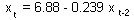
t-ratio = 1.03; P=0.317; = 5.6%. Effect is non-significant! There is nothing to validate. We can stop at this point and say that there is not enough data for validation. However we can make another try and separate the data in a different way. In our case, population numbers in year t depends on population numbers in tear t-2. Thus, we can estimate the regression using uneven years only and then test it using even years.

Regression obtained from uneven years:

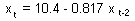
t-ratio = 13.14; P<0.001; = 66.4%. Effect is highly significant.

Now we test this equation using data for even years. The equation is a predictor of population numbers; thus estimated values from the equation can be used as the independent variable and actual population numbers are used as a dependent variable. Then:
R-square = 0.0001
F = 0.0002
P = 0.96
This means that the equation derived from uneven years did not help to predict population dynamics in even years.
Conclusion: the model is not valid.

Crossvalidation

The idea of crossvalidation is to exclude one observation at a time when estimating regression coefficients, and then use these coefficients to predict the excluded data point. This procedure is repeated for all data points, and then, estimated values can be compared with real values. However, I don't know any methods for testing statistical significance with crossvalidation. Standard ANCOVA cannot be applied because it does not account for the variation in regression parameters when some data are not used in the analysis.

Crossvalidation method is often considered as a very economical validation method because it uses the maximum possible observation points for estimating the regression. But, this is wrong! Crossvalidation is NOT A VALIDATION METHOD. It evaluates the variability of regression results when some data from the given set are omitted. This method does not attempt to predict the variability of regression results in other possible data sets characterized by the same autocorrelation.

Jackknife method (Tukey)

Jackknife method is similar to crossvalidation, but its advantage is that it can be used for testing the significance of regression. Details of this method can be found in Sokal and Rohlf (1981. Biometry). Let us consider the same example of colored fox. We need to test if the effect of population density in year t-2 is significant. Jackknife method is applied as follows:

Step 1. Each data point is left out from the analysis in turn, and the regression is estimated each time (same as in crossvalidation). When observation i is excluded we get the equation: 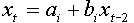. The slope bi characterizes the effect of population density in year t-2 on the population density in year t. Slopes appear to be different for different i, and different from the slope estimated from all data points (b = -0.412). The variability of bi corresponds to the accuracy of estimated slope.

Year, t	xt-2	xt	i	bi	Bi
3	6.562	5.952	1	-0.430	0.286
4	7.318	4.343	2	-0.361	-2.429
5	5.729	6.562	3	-0.435	0.446
6	6.540	7.318	4	-0.530	4.184
7	4.813	5.729	5	-0.407	-0.611
8	5.131	6.540	6	-0.412	-0.429
9	6.605	4.813	7	-0.395	-1.099
10	4.525	5.131	8	-0.427	0.172
11	5.036	6.605	9	-0.409	-0.533
12	5.578	4.525	10	-0.426	0.11
13	6.657	5.036	11	-0.398	-0.962

Step 2. We need to determine if the slope significantly differs from 0 (in our case significantly < 0). But the variation of bi is much smaller than the accuracy of the slope because each slope was estimated from a large number of data points. Thus, we will estimate pseudovalues Bi using the equation:

Bi = Nb - (N - 1)bi

where b = -0.412 is the slope estimated from all data, N is the number of observations, and bi is the slope estimated from all observations except the i-th observation.

Step 3. The last step is to estimate the mean, SD, SE, and t for pseudovalues:

M = -0.403 SD = 1.05 SE = 0.166

t = |SE/M| = 2.43 P = 0.02.

Conclusion: The slope is significantly < 0.

The jackknife procedure is not a validation method for the same reasons as the crossvalidation. However, jackknife is less sensitive to the shape of the distribution than the standard regression. Thus it is more reliable.

Correlogram product method

This is a new method which can be used for validating correlations between population density and other factors. However, this method cannot be used for autoregressive models and thus we cannot apply it for the colored fox example.

This method was developed by Clifford et al. (1989, Biometrics 45: 123-134). The null hypothesis is that variables X and Y are independent but each of them is autocorrelated. For example, if we consider the relationship between population density and solar activity, both variables are autocorrelated. The autocorrelation in population density may result from the effect of solar activity or from other factors, e.g., interaction with predators. In our null hypothesis we consider that solar activity has no effect on the population density, but we allow autocorrelations in the population density.

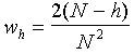
In short, the standard deviation of the correlation between 2 independent autoregressive processes, X and Y equals the square root of the weighted product of correlograms for variables X and Y:

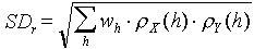
where h is the temporal or spatial lag, are correlograms for variables X and Y, and weights, wh, are equal to the proportion of data pairs separated by lag, h.

Thus, to test for significance of the correlation between processes X and Y we need to estimate the standard error using the equation above. If the absolute value of empirical correlation is larger than SD multiplied by 2 (t-value), then the correlation is significant.

Example. The correlation between log area defoliated by gypsy moth in CT, NH, VT, MA, ME, and NY and the mean number of sunspots in 1964-1994 was r = 0.451:

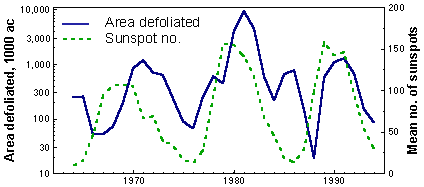
This correlation is significant (P = 0.011), and it seems that we can use solar activity as a good predictor of gypsy moth outbreaks. However, both variables are autocorrelated, and thus, we will use the correlogram product method. Correlograms (=autocorrelation functions, ACF) for both variables are shown below:

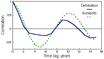
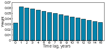
Correlograms are periodic indicating a cyclic behavior of both variables. The cycle is very similar and the period is 9-10 years (location of the first maximum). The weights wh are the following: wo = 1/N, and

for h > 0, where N = 31 is the number of observations:

Now we apply the correlogram product method: multiply both correlograms and weights at each lag, h, and then take the square root from their sum (here we used only for h $lt; 16). The standard error for correlation is SE= 0.337; t = r/SE = 0.451/0.337 = 1.34; P = 0.188.
Conclusion: Correlation between the area defoliated by the gypsy moth and solar activity may be coincidental. More data is needed to check the relationship.

Another possible way of the analysis is autoregression combined with external factors. For example, we can use the model:

where Dt is the area defoliated in year t, Wt is the averrage number of sunspots in year t, and bi are parameters. The error probability (P) for the effect of sunspots will be very close to that obtained in tyhe previous analysis. However, coefficients bi do not necessary have biological meaning. For example, the equation above assums that current defoliation depends on defoliation in previous years, but there may be no functional relationship between areas defoliated in different years. Their correlation may simply result from the effect of some external autocorrelated factor (e.g. solar activity). Thus, it is necessary to use caution in the interpretation of autoregressive models.

Note: In many cases, the effect of a factor is significant with one combination of additional factors but becomes non-significant after adding some more factors. People often select arbitrarily some combination of factors that will maximize statistical significance of the factor tested. However, this is just another way of cheating. If additional factors destroy the relationship between variables that you want to prove, then there is no relationship. It is necessary to use as many additional factors as possible including autoregressive terms.

The sequence of statistical analysis

1. Data collection. Select the population characteristic to measure, select factors that may affect population dynamics, make sure that these factors are measurable with resources available. If you analyze historical data, try to find all data that may be useful for the period of time and area you are interested in. Suggest hypothetical equations that can be useful for analysis.
2. Selection of model equation. Try to incorporate all available data.
3. Regression analysis. Remove factors which effect is not significant. Significance of individual factors is evaluated using sequential regression.
4. Plot residuals versus each factor, check for non-linear effects. If non-linear effects are found, modify the model and go to #3.
5. Validate the model using independent data, or use the correlogram-product method. If the model is valid, then use it. If there is not enough data for validation: use the model with caution (it might be wrong!); collect additional data for validation. If additional data does not support the model, then go to #2.