4.3. Example: Colored fox in Labrador (1839-1880)

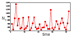
First step is to log-transform the data. When predicting population density, log-transformation is always better than no transformation.

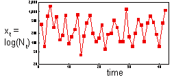
The distribution of log-transformed data is more symmetric now. We will experiment with different factors trying to get the most accurate prediction of log population density.

1. One factor: previous year population counts

Predictor	t-ratio	P
Xt-1	0.25	0.801 NS

= 0.2%.
This means that our regression does not work any better than using average log-density.

2. Two factors: population counts in two previous years

Predictor	t-ratio	P
Xt-1	0.35	0.728 NS
Xt-2	2.73	0.010

= 16.8%.
Effect of year t-1 is not significant, but the effect of year t-2 is significant. Non-significant effect can be ignored. Thus, we can re-estimate regression using year t-2 as the only predictor:

Predictor	t-ratio	P
Xt-2	2.75	0.009

= 16.6%.

3. Plotting the regression

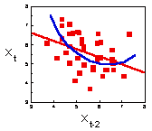
It is always necessary to plot the regression to see if there are any non-linear effects. It seems that some non-linearity may be present (blue line). Let us test for quadratic effects of year t-2.

Predictor	t-ratio	P
Xt-2	1.37	0.179 NS
	1.14	0.261 NS

= 19.4%.
OK, there are no quadratic effects of year t-2.

4. Adding year t-3.
Now we can try to add year t-3. May be the model will work better.

Predictor	t-ratio	P
Xt-2	2.88	0.007
Xt-3	0.41	0.683 NS

= 18.9%.
The model did not get significantly better after adding year t-3 as a predictor. Thus, we cannot improve the model any further.

5. Plotting the residuals.
Now we can plot the residuals () versus population counts in year t-1 to test if there is any non-linear effect of year t-1.

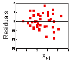
This graph indicates no non-linear effects of population counts in year t-1

6. Prediction of population numbers
Now, we can use the model to predict fox counts a year ahead (t) using population counts in the previous year (t-2) as a predictor:

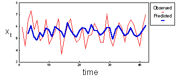
Predicted population counts follow the same pattern as observed values. However, predicted values have smaller variation because any regression has a "smoothing" effect.

In the previous graph, we predicted population counts one year ahead at a time. Let's see what happen if we try to predict the entire time series from two initial values. In this case, the error will propagate because we will use predicted population counts as the base for further predictions.

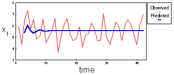
Predicted population counts exhibit damped oscillations. After a few oscillations, they approach the equilibrium level of x=5.553.

This model cannot be used to predict population numbers more than 1-3 years ahead.