4.2. Correlation between factors

First, I will remind you the basics of the analysis of variances (ANOVA)
Total sum of squares (SST) is the sum of squared deviations of individual measurements from the mean. The total sum of squares is a sum of 2 portions:
(1) Regression sum of squares (SSR) which is the contribution of factors into the variance of the dependent variable, and
(2) Error sum of squares (=residual sum of squares) (SSE) which is the stochastic component of the variation of the dependent variable.

SSR is the sum of squared deviations of predicted values (predicted using regression) from the mean value, and SSE is the sum of squared deviations of actual values from predicted values.

The significance of regression is evaluated using F-statistics:

where
df(SSR)= g - 1 is the number of degrees of freedom for the regression sum of squares which is equal to the number of coefficients in the equation, g, minus 1;
df(SSE)= N - g is the number of degrees of freedom for the error sum of squares which is equal to the number of observations, N, minus the number of coefficients, g;
df(SST) = df(SSR) + df(SSE) = N - 1 is the number of degrees of freedom for the total sum of squares.

The null-hypothesis is that factors has no effect on the dependent variable. If this is true, then the total sum of squares is approximately equally distributed among all degrees of freedom. As a result, the fraction of the sum of squares per one degree of freedom is approximately the same for regression and error terms. Then, the F-statistic is approximately equal to 1.

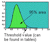
Now, the question is, how much should the F-statistic deviate from 1 to reject the null hypothesis. To answer this question we need to look at the distribution of F assuming the null hypothesis:

If estimated (empirical) value exceeds the threshold value (which corresponds to the 95% cumulative probability distribution) then the effect of all factors combined is significant. (See tables of threshold values for P = 0.05, 0.01, and 0.001)

Note: In some statistical textbooks you can find a two-tail F-test (5% area is partitioned into two 2.5% areas at both, right and left tails of the distribution). This is a wrong method because small F indicates that the regression performs too well (some times suspiciously well). Null hypothesis is not rejected in this case! If F is very small, then we may suspect some cheating in data analysis. For example, this may happen if too many data points were removed as "outliers". However, our objective here is not to test for cheating (we assume no cheating). Thus we use a 1-tail F-test.

The F-distribution depends on the number of degrees of freedom for the numerator [df(SSR)] and denominator [df(SSE)].

Standard regression analysis generally cannot detect the significance of individual factors. The only exception are orthogonal plans in which factors are independent (=not correlated). In most cases, factors are correlated, and thus, a special method called step-wise regression should be used to test the significance of individual factors. The step-wise regression is a comparison of two regression analyses:
(1) the full model and
(2) the reduced model in which one factor is excluded.
The full model has more degrees of freedom, and therefore, it fits data better than the reduced model. Thus, the regression sum of squares, SSR, is greater for the full model than for the reduced model. The question is: is this difference significant or not? If it is not significant, then the factor that was excluded is not important and can be ignored. The significance is tested with the same F-statistic, but SSR and df(SSR) are replaced by the difference in SSR and df(SSR) between the full and reduced models:

where SSR and SSR1 are regression sum of squares for the full and reduced models, respectively; df(SSR) and df(SSR1) are degrees of freedom for the regression sum of squares in the full and reduced models, respectively; SSE is the error sum of squares for the full model; and df(SSE) is the number of degrees of freedom for the error sum of squares.

Because only one factor was removed in the reduced model,

df(SSR) - df(SSR1) = 1.

The F-statistic is related to the t-statistic if the denominator has only one degree of freedom:

Thus, the t-statistic can be used instead of the F in the step-wise regression.

Example of the step-wise regression:
Full model ; SSR =53.2, SSE =76.3, df(SSR) =2, df(SSE) =53.
Reduced model y = a + b x; SSR =45.7, SSE =83.8, df(SSR1)=1, df(SSE1)=54.
F=(53.2-45.7)53 / 76.3 = 5.21; t = 2.28; P<0.05.
Thus, the quadratic term is significant (non-linearity test).