4.6. Biological interpretation of Stochastic Models. Response surfaces.

But, it is possible to modify stochastic models so that they will have some biological interpretation. Usually this modification does not reduce the fit of the model. Let us consider the dynamics of a population with discrete generations (e.g., a monovoltine insect). Population density, Nt in year t can be estimated from population density in the previous year t-1:

where s is survival and F is fecundity. Both, survival and fecundity may depend on the density of the population in year t-1 and on environmental conditions in that year. Survival may also depend on the density of natural enemies (predators, parasites, and pathogens) in year t-1, which may depend on the density of the prey (host) population in year t-2. Thus, survival, s, in year t-1 may be a function of population density in year t-2. Weather conditions in year t-2 may also affect the survival. It is possible to imagine even longer feed-back loops. For example, if it takes 3 years for host plants to recover after severe defoliation caused by insect outbreak, then the quantity and/or quality of food will cause a 3-yr delayed feedback to the insect population.

These density-dependent processes are often called "regulation". However, this term is very ambiguous and I prefer to avoid it (see Lecture 9).

The product of survival and fecundity in the previous equation is the net rate of population increase, R, which is a function of previous population densities and previous weather conditions:

where wt in year t are weather conditions in year t. For simplicity we will ignore weather conditions, and density effects with delays longer than 2 years. Then the equation will become

After log-transformation it will be:

where . is the rate of population increase in year t which can be positive (if the population grows) or negative (if the population declines). Now, the rate of population increase can be represented as a linear function of population densities in the current and previous years:

This equation is still a statistical model because coefficients bi are estimated using regression analysis. However, this equation has some biological meaning. For example, if the effect of population density on the rate of population increase is not significant then the model becomes equivalent to the exponential model. If population growth declines with increasing current density, b1 < 0, then some non-delayed density-dependent processes should be present (e.g., competition, or pathogen infection), and the model is equivalent to the discrete-time logistic model. If population growth declines with increasing density in the previous generation, b2 < 0, then some non-delayed density-dependent processes are present, e.g., parasitism by specialized parasitoids. Delayed density-dependence usually yields oscillations in population density.

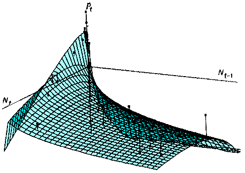
In a more general case, the function is non-linear. It can be represented as some surface in a 3-d space:

Turchin and Taylor (1993, Ecology, 73: 289-305) suggested the following equation for fitting non-linear surfaces:

where bi, h and g are parameters which can be fit using non-linear regression.

Note, that population densities are not log-transformed in the right side of the equation. However, it can be proved that log-transformation is equivalent to setting parameters h or g close to zero. Thus, log-transformation can be considered is a specific case of power-transformation when the power is close to zero.

This is called "response-surface methodology" which means that the shape of the surface is more important than the equation that fits it. Different species may have different response surfaces which can be found using this general equation. Response surface cannot identify mechanisms of population change, but it can indicate some characteristics of these mechanisms, e.g. immediate density-dependence, delayed density-dependence, etc.

Example. Let us analyze the dynamics of colored fox. This time we will predict the rate of population increase rather than population density. First we will use the linear equation that relates the rate of population increase in year t to log-transformed population densities in years t and (t-1):

where . After estimating regression parameters the equation becomes .

Predictor	t-ratio	P
xt	6.93	0.000
xt-1	2.73	0.010

= 76.8%.

The effect of log population numbers in year t-1 on the rate of population increase in year t is the same as the effect of log population numbers in year t-2 on the log population numbers in year t (see our previous example). However, we got a significant effect of population numbers in year t on the rate of population increase in the same year which seems contradict to our previous result that population numbers in year t did not correlate significantly with population numbers in the previous year.

However, there is nothing wrong here. Be got different answers because we asked different questions. In our previous analysis we wanted to know is it possible to improve the prediction of population density in year t using the information about population numbers in the previous year, and we got the negative answer. Then we asked if the rate of population increase is related to the current population density (test for density-dependence) and got a positive answer.

To understand the difference, imagine a perfect density-dependence which draws population density exactly to the equilibrium state. We will also assume that environmental fluctuations add some noise into population dynamics. In this case, population density in year t is just a random variable entirely independent from population density in previous years. But this is the result of a strong density-dependence.

The advantage of using the rate of population increase is in the possibility of interpreting data in terms of density-dependence. Now we can say that there is a non-delayed density-dependence which may be associated with intraspecific competition or pathogens plus delayed density-dependence which may be associated with specialized predators or parasitoids. Finally we will try to improve our model using the method of Turchin and Taylor (1993). Using non-linear regression we get the following equation:

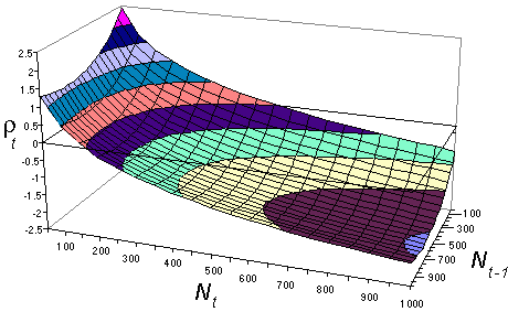
where g = 0.0025 and h = 0.824. = 79.2%. Non-significant terms were remover from the equation of Turchin and Taylor. Prediction has improved a little. The shape of this response surface is shown below:

There is a strong non-delayed density-dependence (effect of Nt) and also some delayed density-dependence (effect of Nt-1) which becomes weaker when density increases.