Age-dependent life-tables

Example. Consider a sheep population which is censused once a year immediately after breeding season:

Age, years (x)	Probability of surviving to age x (lx)	No. of female offspring born to a mother of age x (mx)
0	1.000	0.000
1	0.845	0.045
2	0.824	0.391
3	0.795	0.472
4	0.755	0.484
5	0.699	0.546
6	0.626	0.543
7	0.532	0.502
8	0.418	0.468
9	0.289	0.459
10	0.162	0.433
11	0.060	0.421

Only females are considered in this life-table. However, there is no problem to include male populations into the life table. Then, survival rates should be specified separately for males and females, and the sex ratio of offspring should be taken into account.

Survivorship curves

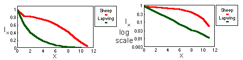
Survivorship curve is exponential (with negative growth) for the lapwing. This means that survival rate is independent of age. In the log-scale, survivorship curve becomes a straight line (see above).

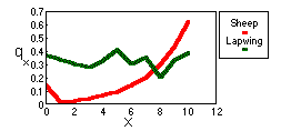
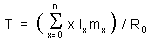
Age-specific mortality is estimated using equation:

Sheep mortality generally increases with age; and the slope of survivorship curve becomes steeper to the end. Humans have a similar shape of survivorship curve.

Characteristics derived from life-tables

In our example, R0 = 1×0 + 0.845×0.045 + 0.824×0.391 + ... = 2.513. It means that an ewe produces 2.513 ewe lambs in average in a lifetime.

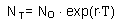
Average generation time, T, is estimated using equation:

In our example, T = (0×1×0 + 1×0.845×0.045 + 2×0.824×0.391 + ...) / 2.513 = 12.825 / 2.513 = 5.1 years. It means that the average age of mothers when they give birth to an eve lamb is 5.1 years.

Note: If organisms breed continuously, then generation time will be overestimated using this equation because all births are summed over the period between census dates which is equal to one age step. Generation time can be adjusted by subtracting half of age step.

Now it is possible to estimate approximate value of intrinsic rate of increase r using the following logic. We assume discrete generations with generation time T=5.1 years and net reproductive rate of R0 =2.513. If population size at zero time was N0, then after T years, the population will grow to NT = N0×R0. According to an exponential model,

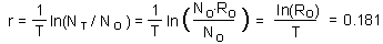
where ln is natural logarithm (logarithm with base e =2.718). We got the equation for r:

Note: This is an approximate estimation of r because we used a simplified assumption that generations are discrete. Accurate estimation of r will be discussed in the next chapter.

Time units used for age measurement

If survival or reproduction are cyclic (e.g., seasonal), then one cycle can be taken as a time unit. In this case it may happen that the number of age intervals will drop to 2 or 3. However, it may be not very dangerous if reproduction is limited to a short period within the year because there will be little age difference between organisms born in the same year.

If survival and reproduction are cyclic but the entire life span is less or equal to this cycle, then time units should be smaller than the cycle length. Age-dependent life-tables can be built for the entire population only if the breeding period is short and therefore organisms' development is synchronized. Otherwise, separate life-tables should be built for subpopulations that start their development at different seasons.

Determining survival of organisms till age x (lx)

This kind of analysis is usually impossible in populations of moving organisms. There are two principal methods to deduce lx values in this case: by determining the age distribution in the population, or by determining the ages at death.

If the population is stationary (i.e., population numbers and age distribution do not change) then the number of new-born organisms x time units ago was the same as now; and survivors of that group of organisms are of age x. Thus,

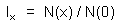
where N(x) is the number of organisms of age x. Here we assumed that age can be accurately measured. In many species the number of "growth rings" in specific organs is equal to age in years. Examples of such organs are: stems of trees, scales of fishes, horns in sheep, roots of canine teeth in bears, otholits in fishes. The weight of the eye lens can be used for age measurement in some animal species. However, in many populations, measuring age is a difficult problem.

Assumption of population stationarity usually is taken a-priori if no historical data exist. In cases when age distribution has a periodic component, we can speculate that it resulted from fluctuations in population numbers. Periodic component can be filtered out using regression methods.

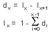
Consider a large number of carcasses whose age have been determined. We assume that the probability of detecting a carcass does not depend on the age of animal at death. The proportion of individuals that were at age x when they died is dx. These individuals survived to age x but did not survive to age x+1. Thus,

The method of estimation of lx from age of carcasses also requires stability of population numbers and of age structure.

Determining reproduction rates (mx)

Reproduction rates are easy to determine in laboratory reared animals or plants. In natural populations of mammals, maternal frequencies can be derived from the proportion of pregnant and/or lactating animals. In birds, maternal frequencies can be determined from the average number of chick per nest. Indirect measures of maternal frequencies should be used with caution because they may be biased.