Stage-dependent life-tables

• The life-cycle is partitioned into distinct stages (e.g., eggs, larvae, pupae and adults in insects)
• Survival and reproduction depend more on organism stage rather than on calendar age
• Age distribution at particular time does not matter (e.g., there is only one generation per year)

Example. Gypsy moth (Lymantria dispar L.) life table in New England (modified from Campbell 1981)

Stage	Mortality factor	Initial no. of insects	No. of deaths	Mortality (d)	Survival (s)	k-value [-ln(s)]
Egg	Predation, etc.	450.0	67.5	0.150	0.850	0.1625
Egg	Parasites	382.5	67.5	0.176	0.824	0.1942
Larvae I-III	Dispersion, etc.	315.0	157.5	0.500	0.500	0.6932
Larvae IV-VI	Predation, etc.	157.5	118.1	0.750	0.250	1.3857
Larvae IV-VI	Disease	39.4	7.9	0.201	0.799	0.2238
Larvae IV-VI	Parasites	31.5	7.9	0.251	0.749	0.2887
Prepupae	Desiccation, etc.	23.6	0.7	0.030	0.970	0.0301
Pupae	Predation	22.9	4.6	0.201	0.799	0.2242
Pupae	Other	18.3	2.3	0.126	0.874	0.1343
Adults	Sex ratio	16.0	5.6	0.350	0.650	0.4308
Adult females		10.4
TOTAL			439.6	97.69	0.0231	3.7674

Specific features of stage-dependent life tables:

• There is no reference to calendar time. This is very convenient for the analysis of poikilothermous organisms.
• Gypsy moth development depends on temperature but the life table is relatively independent from weather.
• Mortality processes can be recorded individually and thus, this kind of life table has more biological information than age-dependent life tables.

K-values

Mortality percentages are not additive. For example, if predators alone can kill 50% of the population, and diseases alone can kill 50% of the population, then the combined effect of these process will not result in 50+50 = 100% mortality. Instead, mortality will be 75%!

Survival is a probability to survive, and thus we can apply the theory of probability. In this theory, events are considered independent if the probability of the combination of two events is equal to the product of the probabilities of each individual event. In our case event is survival. If two mortality processes are present, then organism survives if it survives from each individual process. For example, an organism survives if it was simultaneously not infected by disease and not captured by a predator.

Assume that survival from one mortality source is s1 and survival from the second mortality source is s2. Then survival from both processes, s12, (if they are independent) is equal to the product of s1 and s2:

This is a "survival multiplication rule". If survival is replaced by 1 minus mortality [s=(1-d)], then this equation becomes:

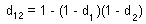
For example, if mortality due to predation is 60% and mortality due to diseases is 30%, then the combination of these two death processes results in mortality of d = 1-(1-0.6)(1-0.3)=0.72 (=72%).

Varley and Gradwell (1960) suggested to measure mortality in k-value which is the negative logarithms of survival:

We use natural logarithms (with base e=2.718) instead of logarithms with base 10 used by Varley and Gradwell. The advantages of using natural logarithms will be shown below.

It is easy to show that k-values are additive:

The k-values for the entire life cycle (K) can be estimated as the sum of k-values for all mortality processes:

In the life table of the gypsy moth (see above), the sum of all k-values (K = 3.7674) was equal to the k-value of total mortality.

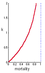This graph shows the relationship between mortality and the k-value. When mortality is low, then the k-value is almost equal to mortality. This is the reason why the k-value can be considered as another measure of mortality. However, at high mortality, the k-value grows much faster than mortality. Mortality cannot exceed 1, while the k-value can be infinitely large.

The following example shows that the k-value represents mortality better than the percentage of dead organisms: One insecticide kills 99% of cockroaches and another insecticide kills 99.9% of cockroaches. The difference in percentages is very small (<1%). However the second insecticide is considerably better because the number of survivors is 10 times smaller. This difference is represented much better by k-values which are 4.60 and 6.91 for the first and second insecticides, respectively.

Key-factor analysis Varley and Gradwell (1960) developed a method for identifying most important factors "key factors" in population dynamics. If k-values are estimated for a number of years, then the dynamics of k-values over time can be compared with the dynamics of the generation K-value. The following graph shows the dynamics of k-values for the winter moth in Great Britain.

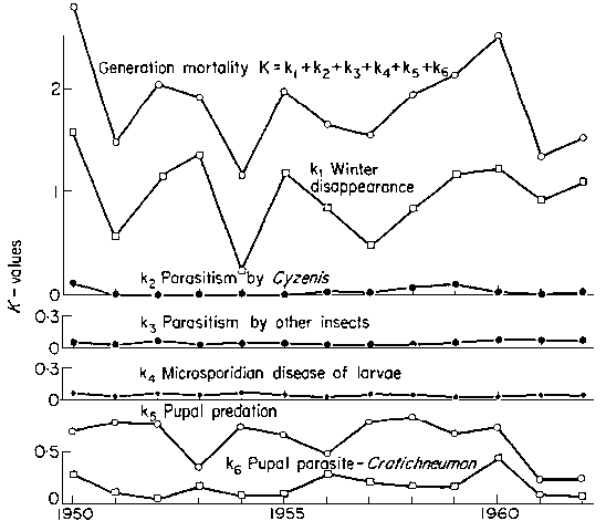
It is seen that the dynamics of winter disappearance (k1) is most resembling the dynamics of total generation K-value. The conclusion was made that winter disappearance determines the trend in population numbers (whether the population will grow or decline), and thus, it can be considered as a "key factor". There were numerous attempts to improve the method. For example, Podoler and Rogers (1975, J. Anim. Ecol, 44(1)) suggested regressing k over K.

But, this method was criticized recently because the meaning of a "key" factor was not explicitly defined (Royama 1996, Ecology). It is not clear what predictions can be made from the knowledge that factor A is a key-factor. For example, the knowledge of key-factors does not help us to develop a new strategy of pest control.

The key-factor analysis was often considered as a substitute for modeling. It seems so easy to compare time series of k-values and to find key-factors without the hard work of developing models of ecological processes. However, reliable predictions can be obtained only from models.

This critique does not mean that life-tables have no value. Life-tables are very important for gathering information about ecological processes which is necessary for building models. It is the key-factor analysis that has little sense.

K-value = instantaneous mortality rate multiplied by time. A population that experience constant mortality during a specific stage (e.g., larval stage of insects) change in numbers according to the exponential model with a negative rate r. We cannot call r intrinsic rate of natural increase because this term is used for the entire life cycle, and here we discuss a particular stage in the life cycle. According to the exponential model:

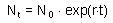
Population numbers decrease and thus, Nt < N0. Survival is: s = Nt/N0 . Now we can estimate the k-value:

Instantaneous mortality rate, m, is equal to the negative exponential coefficient because mortality is the only ecological process considered (there is no reproduction):

Exponential coefficient r is negative (because population declines), and mortality rate, m, is positive.

We proved that if mortality rate is constant, then k-value is equal to the instantaneous mortality rate multiplied by time. This is analogs to physics: distance is equal to speed multiplied by time. Here, instantaneous mortality rate is like speed, and k-value is like distance. K-value shows the result of killing organisms with specific rate during a period of time. If the period of time when mortality occurs is short then the effect of this mortality on population is not large.

If instantaneous mortality rate changes with time, then the k-value is equal to its integral over time. In the same way, in physics, distance is the integral of instantaneous speed over time.

Example. Annual mortality rates of oak trees due to animal-caused bark damage are 0.08 in the first 10 years and 0.02 in the age interval of 10-20 years. We need to estimate total k-value (k) and total mortality (d) for the first 20 years of oak growth.

Thus, total mortality during 20 years is 63%.

Limitation of the k-value concept. All organisms are assumed to have equal dying probabilities. In nature, dying probabilities may vary because of spatial heterogeneity and individual variation (both inherited and non-inherited).

Estimation of k-values in natural populations. Estimation of k-values for individual death processes is difficult because these processes often go simultaneously. The problem is to predict what mortality could be expected if there was only one death process. In order to separate death processes it is important to know the biology of the species and its interactions with natural enemies. Below you can find several examples of separation of death processes.

Example #1. Insect parasitoids oviposit on host organisms. Parasitoid larva hatches from the egg and starts feeding on host tissue. Parasitized host can be alive for a long period. Finally, it dies and parasitoid emerges from it. Insect predators usually don't distinguish between parasitized and non-parasitized prey. If an insect was killed by a predator, then it is usually impossible to detect if this insect was parasitized before. Thus, mortality due to predation is estimated as the ratio of the number of insects numbers destroyed by predators to the total number of insects, whereas mortality due to parasitism is estimated as the ratio of the number of insects killed by parasitoids to the number of insects that survived predation. In this example, predation masks the effect of parasitism, and thus, insects killed by predators are ignored in the estimation of the rate of parasitism. The effect is the same as if predation occurred before parasitism in the life cycle. Thus, in the gypsy moth life table, predation was always considered before parasitism. Diseases also mask the effect of parasitism and thus they are considered before parasitism.

Example #2. It is often possible to distinguish between organisms destroyed by different kinds of predators. For example, small mammals and birds open sawfly cocoons in a different way. Suppose, 20% of cocoons were opened by birds, 50% were opened by mammals, and remaining 30% were alive. The question is what would be the rate of predation if birds and mammals were acting alone. We assume that sawfly cocoons have no individual variation in predator attack rate, and that cocoons destroyed by one predator cannot be attacked by another predator. First, we estimate total k-value for both predator groups: k12 = -ln(0.3) = 1.204. Second, we subdivide the total k-value into two portions proportionally to the number of cocoons destroyed by each kind of predator. Thus, for birds k1 = 1.204×20/(20+50) = 0.344, and for mammals k2 = 1.204×50/(20+50) = 0.860. The third step is to convert k-values into expected mortality if each predator was alone: for birds d1 = 1- exp(-0.344) = 0.291, and for mammals d2 = 1- exp(-0.860) = 0.577.