9.4. Quantitative Measures of Stability
In the previous section we have discussed qualitative indicators of stability. According to these indicators, a model is either stable if its trajectory converges to an equilibrium state or unstable if it diverges from the equilibrium after small disturbances. However, real populations never converge to an equilibrium because of the random noise associated with weather and other stochastic factors. Thus, qualitative stability has a vague biological meaning. Ecologists are more interested in quantitative indicators of stability which represent the ability of the population to resist environmental fluctuations.Robert May (1973) suggested to measure system stability by the maximum real part of eigenvalues of the linearized model. It was shown that this value correlates with the variance of population fluctuations in stochastic models.
Sharov (1991, 1992) suggested measures of m- and v-stability that characterize the stability of the mean (m) and variance (v) of population density (initially these measures were called as coefficients of buffering and homeostasis, see Sharov [1985, 1986]). Later they were re-invented by Ives (1995a, 1995b). They can be used to predict the effect of environmental changes (e.g., global warming or pest management) on the mean and variance of population numbers
M-stability (MS) was defined as the ratio of the change in mean log population density, N, as a response to the change in mean value of some environmental factor, v.

M-stability is the reciprocal of the sensitivity of mean population density to the mean value of factor v. Log-transformation of population density is important because it makes population models closer to linear.
For example, if v is temperature which is going to change by 2 degrees due to global warming, and log population density per ha (log base e) will increase from 1 to 1.5, then the sensitivity is S=(1.5-1)/2=0.25, and m-stability MS=4. The population with higher m-stability will change less than the population with low m-stability under the same changes in average factors.
Strong population regulation increases m-stability because regulating mechanisms will resist to the changes in population density. Let's assume that regulation is caused by interspecific competition. Then, if conditions become favorable for the population, then the organisms will increase their reproduction rate. However, as population density increases, mortality due to competition increases too and partially compensates increased reproduction rates. If conditions become less favorable, then density will decline and mortality due to competition will decrease and partially compensate the decrease in reproduction rates.
If population dynamics is described by a mathematical model then m-stability can be estimated from that model. The simplest example is the logistic model. Mean population density in the logistic model equals to carrying capacity, K. If the factor v affects K, then  . If the factor v affects population growth rate, r, but does not affect carrying capacity, then mean population density will not respond to factor change, and thus, m-stability will be infinitely large.
V-stability (VS) was defined as a ratio of the variance of additive random noise  to the variance of log population numbers
  :
:

Population that has smaller fluctuations of population numbers than another population that experience the same intensity of additive environmental noise has a higher v-stability. To estimate v-stability in the Ricker's model we can use the linearized model at the equilibrium point:

where N is log population density, and  is the white noise with a zero mean. Noise is not correlated with log population numbers. Thus:


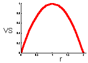
This graph shows that v-stability equals to zero at r=0 and r=2 (these are the boundaries of quantitative stability). V-stability has a maximum at r = 1.
References
Ives, A.R. 1995. Predicting the response of populations to environmental change. Ecology 76: 926-941.
Ives, A.R. 1995. Measuring resilience in stochastic systems. Ecol. Monogr. 65: 217-233.
May, R.M. 1973. Stability in randomly fluctuating versus deterministic environments. Amer. Natur., 107: 621 650.
Sharov, A.A. 1985. Insect pest population management taking into account natural mechanisms of population dynamics. Zoologicheskii Zhurnal (Zoological Journal), 64: 1298 1308 (in Russian).
Sharov, A.A. 1986. Population bufferity and homeastasis and their role in population dynamics. Zhurnal Obshchej Biologii (Journal of General Biology), 47: 183 192 (in Russian).
Sharov, A.A. 1991. Integrating host, natural enemy, and other processes in population models of the pine sawfly. In: Y.N.Baranchikov et al. [eds.] Forest Insect Guilds: Patterns of Interaction with Host Trees. U.S. Dep. Agric. For. Serv. Gen. Tech. Rep. NE-153. pp. 187-198.
Sharov, A.A. 1992. Life-system approach: a system paradigm in population ecology. Oikos 63: 485-494. Get a reprint! (PDF)


