9.3. Equilibrium: Stable or Unstable?

If the dynamics of a system is described by a differential equation (or a system of differential equations), then equilibria can be estimated by setting a derivative (all derivatives) to zero.

Example: Logistic model

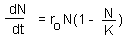
To find equilibria we have to solve the equation: dN/dt = 0:

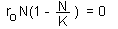
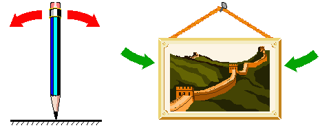
This equation has two roots: N=0 and N=K. An equilibrium may be stable or unstable. For example, the equilibrium of a pencil standing on its tip is unstable; The equilibrium of a picture on the wall is (usually) stable.

An equilibrium is considered stable (for simplicity we will consider asymptotic stability only) if the system always returns to it after small disturbances. If the system moves away from the equilibrium after small disturbances, then the equilibrium is unstable.

The notion of stability can be applied to other types of attractors (limit cycle, chaos), however, the general definition is more complex than for equilibria. Stability is probably the most important notion in science because it refers to what we call "reality". Everything should be stable to be observable. For example, in quantum mechanics, energy levels are those that are stable because unstable levels cannot be observed.

Now, let's examine stability of 2 equilibria points in the logistic model.

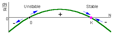
In this figure, population growth rate, dN/dt, is plotted versus population density, N. This is often called a phase-plot of population dynamics. If 0 < N < K, then dN/dt > 0 and thus, population grows (the point in the graph moves to the right). If N < 0 or N > K (of course, N < 0 has no biological sense), then population declines (the point in the graph moves to the left). The arrows show that the equilibrium N=0 is unstable, whereas the equilibrium N=K is stable. From the biological point of view, this means that after small deviation of population numbers from N=0 (e.g., immigration of a small number of organisms), the population never returns back to this equilibrium. Instead, population numbers increase until they reach the stable equilibrium N=K. After any deviation from N=K the population returns back to this stable equilibrium.

The difference between stable and unstable equilibria is in the slope of the line on the phase plot near the equilibrium point. Stable equilibria are characterized by a negative slope (negative feedback) whereas unstable equilibria are characterized by a positive slope (positive feedback).

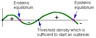
The second example is the bark beetle model with two stable and two unstable equilibria. Stable equilibria correspond to endemic and epidemic populations. Endemic populations are regulated by the amount of susceptible trees in the forest. Epidemic populations are limited by the total number of trees because mass attack of beetle females may overcome the resistance of any tree.

Stability of models with several variables

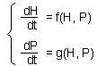
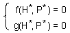
This is the 2-variable model in a general form. Here, H is the density of prey, and P is the density of predators. The first step is to find equilibrium densities of prey (H*) and predator (P*). We need to solve a system of equations:

The second step is to linearize the model at the equilibrium point (H = H*, P = P*) by estimating the Jacobian matrix:

Third, eigenvalues of matrix A should be estimated. The number of eigenvalues is equal to the number of state variables. In our case there will be 2 eigenvalues. Eigenvalues are generally complex numbers. If real parts of all eigenvalues are negative, then the equilibrium is stable. If at least one eigenvalue has a positive real part, then the equilibrium is unstable.

Eigenvalues are used here to reduce a 2-dimensional problem to a couple of 1-dimensional problem problems. Eigenvalues have the same meaning as the slope of a line in phase plots. Negative real parts of eigenvalues indicate a negative feedback. It is important that ALL eigenvalues have negative real parts. If one eigenvalue has a positive real part then there is a direction in a 2-dimensional space in which the system will not tend to return back to the equilibrium point.

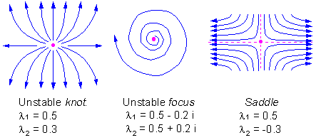
There are 2 types of stable equilibria in a two-dimensional space: knot and focus

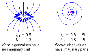
There are 3 types of unstable equilibria in a two-dimensional space: knot, focus, and saddle

Stability in discrete-time models

This model is stable if and only if :

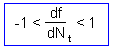
where is the slope of a thick line in graphs below:

You can check this yourself using the following Excel spreadsheet:

Excel spreadsheet "ricker.xls"

If the slope is positive but less than 1, then the system approaches the equilibrium monotonically (left). If the slope is negative and greater than -1, then the system exhibits oscillations because of the "overcompensation" (center). Overcompensation means that the system jumps over the equilibrium point because the negative feedback is too strong. Then it returnes back and again jumps over the equilibrium.

Continuous-time models with 1 variable never exhibit oscillations. In discrete-time models, oscillations are possible even with 1 variable. What causes oscillations is the delay between time steps. Overcompensation is a result of large time steps. If time steps were smaller, then the system would not jump over the equilibrium but will approach to it gradually.

Now we will analyze stability in the Ricker's model. This model is a discrete-time analog of the logistic model:

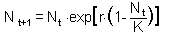
First, we need to find the equilibrium population density N* by solving the equation:

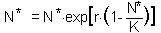
This equation is obtained by substituting Nt+1 and Nt with the equilibrium population density N* in the initial equation. The roots are: N* = 0 and N* = K.. We are not interested in the first equilibrium (N* = 0) because there is no population. Let's estimate the slope df/dN at the second equilibrium point:

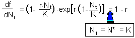
Now we can apply the condition of stability:

Thus, the Ricker's model has a stable equilibrium N* = K if 0 < r < 2.

If a discrete time model has more than one state variable, then the analysis is similar to that in continuous-time models. The first step is to find equilibria. The second step is to linearize the model at the equilibrium state, i.e., to estimate the Jacobian matrix. The third step is to estimate eigenvalues of this matrix. The only difference from continuous models is the condition of stability. Discrete-time models are stable (asymptotically stable) if and only if all eigenvalues lie in the circle with the radius = 1 in the complex plain.