10.4. Predator-Prey Model with Functional and Numerical Responses

We will start with the prey population. Predation rate is simulated using the Holling's "disc equation" of functional response:

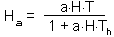
The rate of prey consumption by all predators per unit time equals to

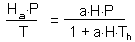
The equation of prey population dynamics is:

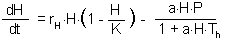
Here we assumed that without predators, prey population density increases according to logistic model.

Predator dynamics is represented by a logistic model with carrying capacity proportional to the number of prey:

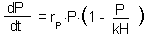
This equation represents the numerical response of predator population to prey density.

The model was built using an Excel spreadsheet:

Excel spreadsheet "predfunc.xls"

You can modify parameters of this model to simulate various patterns of population dynamics. Differential equations are solved numerically, and it may happen that the algorithm (2nd order Runge-Kutta method) will not work for some combination of parameter values. Thus, change parameters with caution. If you suspect that the algorithm does not work properly, reduce the time step (cell A5) until results become independent from the time step.

Simulation results are presented below. This model exhibits more various dynamic regimes than the Lotka-Volterra model.

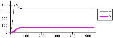	rH = 0.2 K = 500 a = 0.001 Th = 0.5 rP = 0.1 k = 0.2	No oscillations
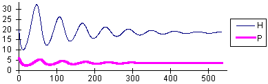	rH = 0.2 K = 500 a = 0.1 Th = 0.5 rP = 0.1 k = 0.2	Damping oscillations converging to a stable equilibrium
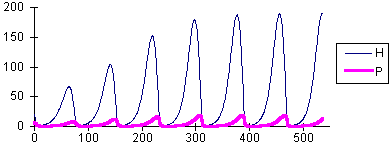	rH = 0.2 K = 500 a = 0.3 Th = 0.5 rP = 0.1 k = 0.2	Limit cycle

This model can be used to simulate biological control. The goal of biological control is to suppress the density of the pest population using natural enemies. We will assume that the prey in our model is a dangerous pest, and that the predator was introduced to suppress its density. Withour predators the density of prey population is equal to the carrying capacity, K = 500. After a predator with a search rate, a = 0.001, was introduced, the equilibrium population density, N^*, declined to the value of 351. Beddington et al. (1978, Nature, 273: 573-579) suggested to measure the degree of pest suppression by the ratio:

.

For example, if a = 0.001, then q = N^*/K = 351/500 = 0.7. Biological control is successful if the value of q is low (at least, <0.5). If we increase the search rate of the predator (i.e., we introduced a more effective predartor species) to a = 0.1, then the pest population is suppressed to the density of 19 (q = 0.038).

It could be expected that more effective predators will cause more suppression of the prey population density. But this is not true, because more effective natural enemies also cause larger oscillations in population density. For example, at a = 0.3, the equailibrium is not stable and populations exhibit periodic cycles (see graph #3 above). Periodically host density reaches the value of 190.

The transition between the stable equilibrium and the limit cycle occurs approximately at a = 0.244. The transition from one type of dynamics to another one is often called "phase transition" (e.g., transitions between liquid and gas phases or between solid and liquid phases). The phase transition in our model will be less ubrupt if we introduce noise. With noise, the system will exhibit oscillations even if the equilibrium is stable. The closer we are to the critical value, a = 0.244, the larger will be these oscillations. These oscillations result from the interaction of predators with prey.

This example illustrates that pest regulation (or control) by natural enemies is an ambibuous notion. First, it does not refer to the type of dynamics (stable equilibrium vs. limit cycle), and second, the excess of "regulation" may cause large oscillations of prey density.