10.3. Functional and Numerical Response
Holling (1959) studied predation of small mammals on pine sawflies, and he found that predation rates increased with increasing prey population density. This resulted from 2 effects: (1) each predator increased its consumption rate when exposed to a higher prey density, and (2) predator density increased with increasing prey density. Holling considered these effects as 2 kinds of responses of predator population to prey density: (1) the functional response and (2) the numerical response.
Modeling Functional Response
Holling (1959) suggested a model of functional response which remains most popular among ecologists. This model is often called "disc equation" because Holling used paper discs to simulate the area examined by predators. Mathematically, this model is equivalent to the model of enzime kinetics developed in 1913 by Lenor Michaelis and Maude Menten.This model illustrates the principal of time budget in behavioral ecology. It assumes that a predator spends its time on 2 kinds of activities:
- Searching for prey
- Prey handling which includes: chasing, killing, eating and digesting.
Total time equals to the sum of time spent on searching and time spent on handling::

Assume that a predator captured Ha prey during time T. Handling time should be proportional to the number of prey captured:

where Th is time spent on handling of 1 prey.
Capturing prey is assumed to be a random process. A predator examines area a per time unit (only search time is considered here) and captures all prey that were found there. Parameter a is often called "area of discovery", however it can be called "search rate" as well.
After spending time Tsearch for searching, a predator examines the area = a Tsearch, and captures aHTsearch prey where H is prey density per unit area:

Hence:

Now we can balance the time budget:

The last step is to find the number of attacked prey Ha:

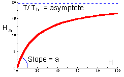
The graph of functional response that corresponds to this equation is shown below:

This function indicates the number of prey killed by 1 predator at various prey densities. This is a typical shape of functional response of many predator species. At low prey densities, predators spend most of their time on search, whereas at high prey densities, predators spend most of their time on prey handling.
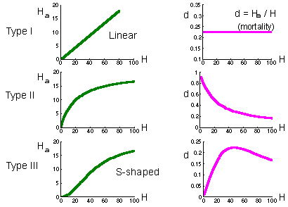
Holling (1959) considered 3 major types of functional response:

Type I functional response is found in passive predators like spiders. The number of flies caught in the net is proportional to fly density. Prey mortality due to predation is constant (right graph on the previous page).
Type II functional response is most typical and corresponds to the equation above. Search rate is constant. Plateau represents predator saturation. Prey mortality declines with prey density. Predators of this type cause maximum mortality at low prey density. For example, small mammals destroy most of gypsy moth pupae in sparse populations of gypsy moth. However in high-density defoliating populations, small mammals kill a negligible proportion of pupae.
Type III functional response occurs in predators which increase their search activity with increasing prey density. For example, many predators respond to kairomones (chemicals emitted by prey) and increase their activity. Polyphagous vertebrate predators (e.g., birds) can switch to the most abundant prey species by learning to recognize it visually. Mortality first increases with prey increasing density, and then declines.
If predator density is constant (e.g., birds, small mammals) then they can regulate prey density only if they have a type III functional response because this is the only type of functional response for which prey mortality can increase with increasing prey density. However, regulating effect of predators is limited to the interval of prey density where mortality increases. If prey density exceeds the upper limit of this interval, then mortality due to predation starts declining, and predation will cause a positive feed-back. As a result, the number of prey will get out of control. They will grow in numbers until some other factors (diseases of food shortage) will stop their reproduction. This phenomenon is known as "escape from natural enemies" discovered first by Takahashi.
Estimation of Parameters of Functional Response
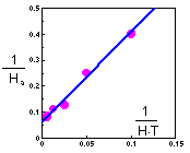
Experiments should be done as follows: predators are kept in large-size cages individually. Large-size cages are important because search abilities of predators should be limited. Different number of prey are released in these cages. Each prey density should be replicated to get sufficient accuracy. More experiments should be done with low prey density than with high prey density because the error of mortality estimates depends on the total number of prey. Experiments are usually set for a fixed time interval. At the end of experiments, survived prey are counted in each cage.This is an example of experimental data:
|
No. of prey per cage H | No. of replications |
Total prey killed | Average no. of prey killed Ha | 1/Ha | 1/(HT) |
| 5 | 20 | 50 | 2.5 | 0.400 | 0.1000 |
| 10 | 10 | 40 | 4.0 | 0.250 | 0.0500 |
| 20 | 7 | 55 | 7.9 | 0.127 | 0.0250 |
| 40 | 5 | 45 | 9 | 0.111 | 0.0125 |
| 80 | 3 | 38 | 12.6 | 0.079 | 0.0062 |
| 160 | 3 | 35 | 11.6 | 0.086 | 0.0031 |
Cage area was 10 sq.m., and duration of experiment was T=2 days. Holling's equation can be transformed to a linear form:

 The linear regression has the following coefficients:
y = 3.43 x + 0.0612
Th = 0.0612 T = 0.1224 days = 2.9 hours
a = 1/3.43 = 0.29 cages = 2.9 sq.m.
Another possible method of parameter estimation is non-linear regression. It may give better results at high prey density than the linear regression method.
Type III functional response can be simulated using the same Holling's equation with search rate (a) dependent on prey density, e.g.:

Numerical Response
Numerical response means that predators become more abundant as prey density increases. However, the term "numerical response" is rather confusing because it may result from 2 different mechanisms:
- Increased rate of predator reproduction when prey are abundant (numerical response per se)
- Attraction of predators to prey aggregations ("aggregational response")
The most simple model of predator's numerical response is based on the assumption that reproduction rate of predators is proportional to the number of prey consumed. This is like conversion of prey into new predators. For example, as 10 prey are consumed, a new predator is born.
Aggregation of predators to prey density is often called "aggregational response". This term is better than "numerical response" because it is not ambiguous. Aggregational response was shown to be very important for several predator-prey systems. Predators selected for biological control of insect pests should have a strong aggregational response. Otherwise they would not be able to suppress prey populations. Also, aggregational response increases the stabilility of the spatially-distributed predator-prey (or host-parasite) system.
References:
Holling, C.S. 1959. The components of predation as revealed by a study of small mammal predation of the European pine sawfly. Canad. Entomol. 91: 293-320.Holling, C.S. 1959. Some characteristics of simple types of predation and parasitism. Canad. Entomol. 91: 385-398.


