12.2. Diffusion Models

where N is population density, and D is diffusion coefficient. This equation indicates that the rate of population change is proportional to the curvature of population density. Examples below show that population increases where curvature is positive and decreases where it is negative.

Skellam (1951) combined diffusion equation in a 2-dimensional space with exponential local population growth:

Model assumptions:

• all individuals simultaneously disperse and reproduce;
• there is no variation in dispersal abilities of individuals.

Skellam's model predicts that if a population was released at a single point, then its spatial distribution will be a 2-dimensional normal distribution:

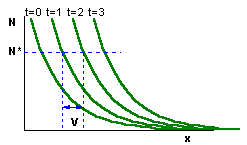
One of the most interesting features of this model is that it predicts the asymptotic rate of expansion of population front. The rate of population expansion, V, is defined as the distance between sites with equal population densities in two successive years:

Skellam's model gives the following equation for the rate of population expansion:

Excel spreadsheet "skellam.xls"

Both parameters, r and D, can be estimated in independent experiments. Intrinsic rate of population increase can be determined from the life-table. Diffusion coefficient D can be estimated using mark-recapture experiments. For example, if marked animals are released within a uniform grid of traps, then diffusion coefficient is estimated as:

where M(t) is mean displacement of organisms recaptured t units time after their release (Skellam 1973).

Example:
The muskrat (Ondatra zibethica) was introduced to Europe in 1905 near Prague. Since that time its area expanded, and the front moved with the rate ranging from 0.9 to 25.4 km/yr. Intrinsic rate of population increase was estimated as 0.2-1.1 per year, and diffusion coefficient ranged from 51 to 230 sq.km/yr. Predicted spread rate (6.4-31.8 km/yr) corresponds well to actual rates of spread.