2.4. Elements of geostatistics
Geostatistics is a collection of statistical methods which were traditionally used in geo-sciences. These methods describe spatial autocorrelation among sample data and use it in various types of spatial models. Geostatistical methods were recently adopted in ecology (landscape ecology) and appeared to be very useful in this new area.Geostatistics changes the entire methodology of sampling. Traditional sampling methods don't work with autocorrelated data and therefore, the main purpose of sampling plans is to avoid spatial correlations. In geostatistics there is no need in avoiding autocorrelations and sampling becomes less restrictive. Also, geostatistics changes the emphasis from estimation of averages to mapping of spatially-distributed populations.
Spatial autocorrelation can be analyzed using correlograms, covariance functions and variograms (=semivariograms). For simplicity, here we will use correlograms only. Covariance functions and variograms are discussed in the next lecture.
In brief, geostatistical analysis usually has the following steps:
- Estimation of correlogram
- Estimation of parameters of the correlogram model
- Estimation of the surface (=map) using point kriging, or
- Estimation of mean values using block kriging
Estimation of Correlogram
Correlogram is a function that shows the correlation among sample points separated by distance h. Correlation usually decreases with distance until it reaches zero. Correlogram is estimated using equation:
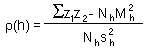
where z1 and z2 are organism numbers in two samples separated by lag distance h, summation is performed over all pairs of samples separated by distance h; Nh is the number of pairs of samples separated by distance h; Mh and sh are the mean and the standard deviation of samples separated by distance h (each sample is weighted by the number of pairs of samples in which it is included).
Notes:
- This is an omnidirectional correlogram; "omnidirectional" means that we don't care about the direction of lag h.
- Serious geostatistical analysis often includes estimation of directional correlograms (see next lecture). It may happen that points are more closely correlated in some direction (e.g., NE-SW) than in other directions. If correlogram depends on direction, then the spatial pattern is called anisotropic. If no anisotropy detected, then it is possible to use the omnidirectional correlogram.
- Correlogram equation works only if there are no trends in population density in the study area. If a trend exists, then a non-ergodic correlogram should be used instead (see next lecture).
Estimation of parameters of correlogram model
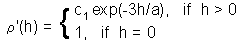
The correlogram can be approximated by some mathematical model. Two models are used most often:1. Exponential model:
2. Spherical model:
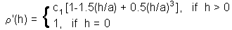
where c1 is sill, and a is range. These parameters can be found using the non-linear regression.
Estimation of the surface (=map) using point kriging (ordinary kriging)
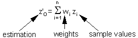
The value z'o at unsampled location 0 is estimated as a weighted average of sample values z2 at locations i around it:
Weights depend on the degree of correlations among sample points and estimated point. The sum of weights is equal to 1 (this is specific to ordinary kriging):

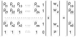
Weights are estimated individually for each point in a regular spatial grid using the system of linear equations:
where  is the Lagrange parameter;
 is the correlation between points i and j which is estimated from the variogram model using distance, h, between points i and j; 0 is the estimated point; 1,...,n are sample points.
Using matrix notation this system can be re-written as:

The solution of this matrix equation is:

Now, weights are found, and thus, it is possible to estimate the value z'o. When these values are estimated for all points in a regular grid, then we get a surface of population density.
The variance of local estimation  is equal to:
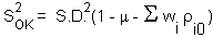
Estimation of the mean value using block kriging
The only difference of block kriging from point kriging is that estimated point (0) is replaced by a block. Consequently, the matrix equation includes "point-to-block" correlations:
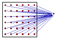
Point-to-block correlation  is the average correlation between sampled point i and all points within the block (in practice, a regular grid of points within the block is used, as shown in the figure).
The variance of block estimation is equal to: 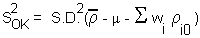
Where  is the average correlation within the block (average correlation between all pairs of grid nodes within the block).
Advantages of kriging:
- It handles spatial autocorrelation
- It is not sensitive to preferential sampling in specific areas
- It estimates both: local population densities and block averages.
- It can replace stratified sampling if the size of aggregations is larger than the inter-sample distance.
References
Isaaks, E. H. and R. M. Srivastava. 1989. An Introduction to Applied Geostatistics. Oxford Univ. Press, New York, Oxford. (a very good introductory textbook)Deutsch, C. V. and A. G. Journel. 1992. GSLIB. Geostatistical software library and user's guide. Oxford Univ. Press, Oxford. (software code written in FORTRAN; I have translated a portion of this library into the C-language).
Geostatistics in ecology (review papers):
Rossi, R. E., D. J. Mulla, A. G. Journel and E. H. Franz. 1992. Geostatistical tools for modelling and interpreting ecological spatial dependence. Ecol. Monogr. 62: 277-314.
Liebhold, A. M., R. E. Rossi and W. P. Kemp. 1993. Geostatistics and geographic information systems in applied insect ecology. Annu. Rev. Entomol. 38: 303-327.


