2.2. Simple Random or Systematic Sampling
Two possible objectives for sampling:- Estimate average population density,
- Make a map of population density.
Moreover, systematic sampling has an advantage over random sampling if the number of samples is large because of more uniform coverage of the entire sampling area. It is especially important for making population maps. Random sampling can be used if the objective is to estimate the mean population density and the number of samples is not large (<100).
Preferential sampling of specific areas (e.g., high-density areas) was always considered unacceptable. However, modern geostatistical methods and stratified sampling can take advantage of preferential sampling. This shows that the methodology of sampling evolves and old textbooks may give obsolete recipes.
Traditional statistical methods include estimation of the mean population density (M), standard deviation (S.D.), and standard error (S.E.), which is the standard deviation of the sample mean.

The equation for standard error is derived assuming that all samples are independent. This is a very strong assumption which is unrealistic in many situations. Samples separated by small distance are often positively correlated. Before using standard statistics it is important to test if samples are correlated. Spatial correlations are examined using geostatistics. The simplest geostatistical test for spatial autocorrelation is the omnidirectional correlogram:

where z1 and z2 are organism numbers in two samples separated by lag distance h, summation is performed over all pairs of samples separated by distance h; Nh is the number of pairs of samples separated by distance h; Mh and sh are the mean and the standard deviation of samples separated by distance h (each sample is weighted by the number of pairs of samples in which it is included).
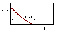
Correlation decreases with distance between samples as shown below.

The range of correlogram is the lag distance h at which correlation reaches (or becomes close to) zero. Standard statistics can be applied only if inter-sample distance exceeds the range of the correlogram.

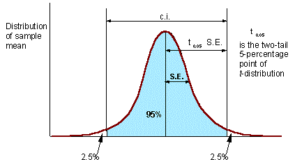
Confidence interval (c.i.) is the interval where the population mean can be found with probability of (1 - P), where P is error probability (e.g., P = 0.05). The number of degrees of freedom d.f. = N - 1 (one d.f. goes for estimation of sample mean).
Precision of sample mean is
There is an empirical rule that precision should be below 0.05 (or 0.1). However, this rule is not universal The only thing that matters in statistics is testing hypotheses. If null-hypothesis is rejected then it does not matter whether A was above or below 0.05. However, in each specific research area, it is useful to find a precision level which is usually sufficient for rejecting null-hypotheses.
Example:. Insect pest population should be suppressed if its density exceeds the economic injury level (EIL). A null-hypothesis is tested that the average density M is equal to EIL. If EIL is within the c.i. for M, then the null-hypothesis cannot be rejected and no decision can be made. In this case, more samples should be taken. If the EIL is outside of the c.i., then null-hypothesis is rejected, and population is suppressed if M > EIL, or not suppressed if M < EIL.


